The secrets of bronze, silver, and gold

Data Ingestion Framework & Medallion Architecture

Introduction

This blog post is the first in a series focused on end-to-end data ingestion and transformation with Databricks, based on the principles of the Medallion architecture. The project will feature the vehicle datasets published by the Dutch RDW (national vehicle authority) and is aimed to exemplify a basic data processing workflow using core Databricks functionalities. In this first blog, we will focus on data ingestion and processing data using the medallion architecture in a bronze-silver-gold layer design. The blog series consists of:

1. The secrets of bronze, silver, and gold (YOU ARE HERE NOW!): Data Ingestion Framework & Medallion Architecture.

2. DQX: We do not trust the data we have not validated: Data Quality Checks with DQX

3. Claude meets JSON: automating Databricks dashboards: Dashboard Automation with Claude Code.

4. You need a companion to explore your data: Companion App for Data Exploration.

5. Deploy your project like a pro with Databricks Asset Bundles.

6. It’s all great, but how much does it cost?: Cost Optimization & Analysis.

---

The framework

Data ingestion forms the foundation of any data engineering process. Broadly speaking, it involves collecting external data to an internal and centralized location, such as the Unity Catalog. Databricks offers various built-in connectors to link external sources to your workspace, but many use cases still warrant custom code implementations.

Figure 1: Data flow from raw ingestion to gold layer in Unity Catalog

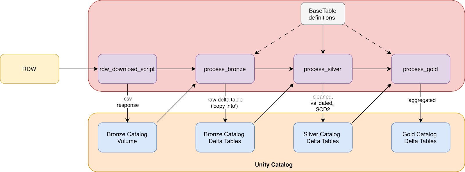
For most data, there is a lot of processing to be done before it is actually ready for production purposes. Raw data often arrives messy and suffers from problems such as inconsistent formats, duplicates, or missing values. A typical processing pipeline follows the three-layer Medallion architecture: bronze, silver and gold. Rather than attempting complex transformations in a single step, each layer adds incremental quality and structure, and breaks the work into manageable stages. In general the Medallion architecture dictates that bronze data is raw and unprocessed, silver data is cleaned and validated, and gold data is aggregated and curated to a business-ready form. Figure 1 displays the dataflow that we adhere to in this project. For more reading material on the Medallion architecture we highly recommend:

• What is the medallion lakehouse architecture? by Databricks

• Building Medallion Architectures: Designing with Delta Lake and Spark, by Piethein Strengholt (2025)

All code and examples are designed to work with the dataset provided by the RDW, as shown in the overview Figure 1. The full code repository can be viewed here. The repo is structured as shown below:

rdw_repo/
  ├── dashboard
  ├── webapp
  ├── src/
  │   └── rdw/
  │       ├── jobs/
  │       ├── dqx_checks/
  │       ├── views/
  │       ├── scd2/
  │       └── utils/
  │
  └── tests/
      ├── fixtures/
      ├── test_data/
      ├── unit_tests/
      └── integration_tests/

The ingestion scripts for the Medallion architecture reside in src/rdw/jobs.

Ingestion

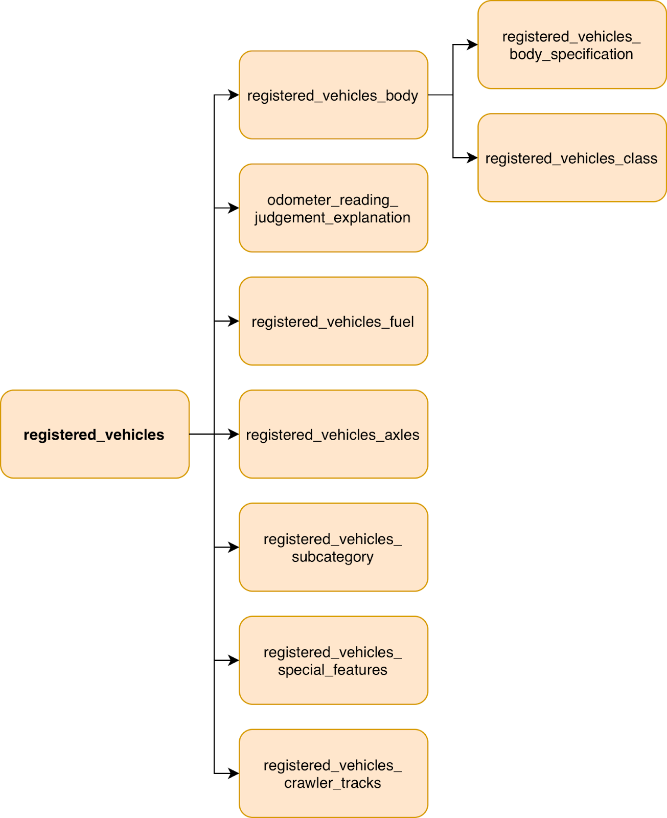
Before actually ingesting any data, we modeled all 10 tables using Pydantic Basetables. This serves multiple purposes: it gives us an internal representation of what the data looks like (and should look like), but also provides a place to define computed properties (e.g., filepaths) that stay consistent across the codebase.

Although Python does offer built-in dataclasses, there are multiple reasons to choose for Pydantic. Pydantic enforces type validation at runtime, catching misconfigurations early rather than letting them emerge further down in the pipeline. It also makes serialization straightforward: table definitions can be exported to YAML or JSON, which becomes useful when you want to version control configurations separately from code or share them across tools. For a project like this, where table definitions drive everything from ingestion to validation to schema creation, having such flexibility is a big advantage.

The structure of the raw RDW tables is shown in Figure 2 below:

Figure 2: Structure of RDW dataset tables

We define the structure of the tables in models.py :

class BaseColumn(BaseModel):
   input_col: str # column names in raw input data
   output_col: str # processed column names
   original_type: Type
   output_data_type: DataType
   is_nullable: bool = True
   is_primary_key: bool = False
   is_foreign_key: bool = False
   foreign_key_reference_table: str = None
   foreign_key_reference_column: str = None


class BaseTable(BaseModel):
   name: str
   description: str
   columns: list[BaseColumn]


class RDWTable(BaseTable):
   url: str
   database: str = “rdw_etl”

Then the actual tables are constructed in definitions.py. Here, input_col denotes the original column name, and output_col is the translated and cleaned column name used in our tables. This is based on the RDWs own documentation of the dataset here (pdf). LLMs and Databricks ai_parse_document() are your friend here to automatically populate the tables!

RDWTable(
 url=”https://opendata.rdw.nl/api/views/m9d7-ebf2/rows.csv?accessType=DOWNLOAD”,
   name=”gekentekende_voertuigen”,
   description=”Main dataset of registered vehicles in the Netherlands. Contains comprehensive vehicle information including registration details, technical specifications, ownership, and inspection data.”,
   columns=[
       BaseColumn(
           input_col=”Kenteken”,
           output_col=”license_plate”,
           original_type=str,
           output_data_type=StringType(),
           is_primary_key=True,
           is_nullable=False,
           description=”The license plate of a vehicle, consisting of a combination of numbers and letters. This makes the vehicle unique and identifiable.”,
       ),
       BaseColumn(
           input_col=”Merk”,
           output_col=”make”,
           original_type=str,
           output_data_type=StringType(),
           description=”The make of the vehicle as specified by the manufacturer.”,
       ),
       BaseColumn(
           input_col=”Handelsbenaming”,
           output_col=”trade_name”,
           original_type=str,
           output_data_type=StringType(),
           description=”Trade name of the vehicle as provided by the manufacturer. May differ from what appears on the vehicle.”,
       ),
       # more columns here ...
   ]
)

Having defined all tables, it is now possible to start the ingestion. In this case, we opted to download raw .csv tables from the RDW dataset. Each table is then sent to a Volume in the bronze layer catalog, using a timestamped folder. In the full implementation timestamps are passed from the job start time environment variable.

def download_table_data(table_name: str, run_timestamp: Optional[str] = None):
   table = get_table_by_name(table_name)
   if not table:
       raise TableNotFoundException(
           f”Table ‘{table_name}’ not found. Available tables: {[t.name for t in rdw_tables]}”
       )


   # Use provided timestamp or generate new one
   timestamp = run_timestamp or datetime.now().strftime(”%Y-%m-%dT%H-%M”)
   destination = table.get_timestamped_volume_path(timestamp)


   chunked_download(table.url, destination)

Bronze

The bronze layer typically contains a copy of the raw source data, with as little as preprocessing as possible. Copying raw data into a table can, for example, be achieved using SQL COPY INTO. In our use case, minimal preprocessing had to be performed as the source tables used whitespaces in the column names, which is not accepted (by default) in Delta tables. This was resolved by using the table.output_col values to rename columns. Consequently, the data was stored into the bronze layer Delta tables.

def transform_bronze(df, table):
   df = convert_columns_from_definition(df, table)
   return df


def process_bronze_layer(table_name: str, run_timestamp: Optional[str] = None):
   table = get_table_by_name(table_name)
   if not table:
       raise TableNotFoundException(
           f”Table ‘{table_name}’ not found. Available tables: {[t.name for t in rdw_tables]}”
       )


   # 1. Read CSV from volume
   if run_timestamp:
       timestamp = run_timestamp # use provided timestamp
   else:
       timestamp = get_latest_timestamp_folder(table.volume_base_path) # auto-detect latest timestamp folder


   source_path = table.get_timestamped_volume_path(timestamp)
   df = read_volume_csv(source_path)


   # 2. Apply bronze transformations
   logger.info(”Applying transformations”)
   df = transform_bronze(df, table)


   # 3. Write to bronze layer
   save_delta_table(df, table.delta_bronze_path)

Silver

Most of the actual data processing happens in the silver layer. In our case, data is cleaned, validated and all of the metadata is added, such as primary/foreign keys, and table/column descriptions. Our data is validated using the DQX - Data Quality Framework by Databricks Labs. Using the create_table_statements function, the PKs, FKs, column types and nullable property are enforced. Then, alter_comments_statements generates SQL statements to set the table and column descriptions.

Table metadata

In the BaseTable class the functions create_table_statement and alter_comment_statements are used to build SQL statements for the table creation and comment setting, respectively. Both are essentially string builders that use information from the table definitions. For example, the comment statements are built using:

def alter_comment_statements(self, catalog: str = bronze_catalog, schema: str = rdw_schema) -> str:
   # Use an array because Spark.SQL() can only process one ALTER statement at a time.
   alter_statements = []


   # Add table-level comment
   table_comment = self.description.replace(”’”, “”)
   alter_statements.append(f’ALTER TABLE {catalog}.{schema}.{self.name} SET TBLPROPERTIES (”comment” = “{table_comment}”);\n’)


   # add comments for each col
   for col in self.columns:
       alter_statements.append(f’ALTER TABLE {catalog}.{schema}.{self.name} ALTER COLUMN {col.output_col} COMMENT “{col.comment}”;\n’)


   return alter_statements

Preparation script

Before running the actual silver processing script, a small preparation script is executed that generates and builds the silver tables with primary keys set. This ensures that all tables are ready to be populated before running the processing step. Foreign keys are set in the processing script itself, as they can only be set after all tables with their primary keys exist.

Data validation

Data validation is the next step in order to ensure the contents of the tables match our expectations and quality standards. Specifically, we validate primary- and foreign keys contents, datetime formats and logic, and null values. All rows that get rejected during validation are placed in a quarantine table such that they can be inspected later, and if necessary, fixed. Our validation rules used the DQX framework and stored the rules in YAML configuration files. More on this in blog post 2!

SCD2

In our project we decided to go with a custom SCD2 implementation. Slowly Changing Dimensions (SCD) provides a solution for handling source data changes over time. The simplest approach is SCD type 1, which simply overwrites old values and is easiest to implement. SCD type 2 preserves history, and instead of overwriting, marks existing record as current or not. In our use case, it allows us to see cars that have been exported or scrapped, and are no longer in the dataset. Whilst useful, SCD2 does pose a trade-off with added complexity.

Databricks offers a few paths for implementing SCD2. Delta Live Tables provides built-in support through the APPLY CHANGES INTO API, but you can also implement it yourself using MERGE statements on standard Delta tables. We opted for a custom implementation as it provides more flexibility in a custom pipeline.

Job script

In the final silver job, the following steps are taken:

• Create and prepare the table with metadata using SQL

• Read from bronze layer

• Apply data validation

• Perform SCD2

• Write to silver layer

The code looks as follows:

def process_silver_layer(table_name: str, full_refresh: bool = False):
   spark = get_spark_session()


   # specify which table is processed
   table = get_table_by_name(table_name)
   if not table:
       raise TableNotFoundException(
           f”Table ‘{table_name}’ not found. Available tables: {[t.name for t in rdw_tables]}”
       )


   # Ensure silver table exists with proper schema
   create_silver_table_if_not_exists(table, spark, logger)


   # 1. Read bronze snapshot and existing silver history
   bronze_data = read_delta_table(table.delta_bronze_path, spark)


   # 2. Apply data quality checks (quarantine is saved internally)
   new_snapshot = apply_dqx_validation(bronze_data, table, logger)


   old_snapshot = None
   if spark.catalog.tableExists(table.delta_silver_path):
       old_snapshot = read_delta_table(table.delta_silver_path, spark)
   # else -> No existing silver history found (first load)


   # 3. Apply SCD2 transformations
   history = transform_silver(new_snapshot, old_snapshot, spark)


   # 4. Write to silver layer
   save_delta_table_preserve_constraints(history, table.delta_silver_path, spark)

Gold

The gold layer typically contains aggregated and joined data. In our case we created a processed table of all registered vehicles. This involved filtering on the following criteria

• Entry is current SCD2 record (`F.col(”__is_current”) == True`).

• Vehicle was not recently exported

• Passenger cars only

• Car is not a taxi

• Is insured and allowed to drive on the road

In addition, a deduplicated table is saved which only contains distinct vehicles (brand/model) and does not contain car-specific information such as MOT expiration. We also construct a metric view which provides an aggregation of the registered vehicle data. The metric view is built from a YAML definition in vehicle_fleet_metrics.yml.

def process_gold_layer():
   spark = get_spark_session()

   # Load
   df = load_silver_registered_vehicles(spark)

   # Transform
   df_main, df_dedup = transform_licensed_vehicles(df)

   # Save tables
   save_delta_table(df_main, f”{gold_catalog}.{rdw_schema}.registered_vehicles”)

   save_delta_table(df_dedup, f”{gold_catalog}.{rdw_schema}.registered_vehicles_dedup”
)
   # Create metric view
   yaml_path = VIEWS_DIR / “vehicle_fleet_metrics.yml”

   yaml_content = load_metric_view_yaml(yaml_path)
   metric_view_name = f”{gold_catalog}.{rdw_schema}.vehicle_fleet_metrics”
   create_metric_view(spark, metric_view_name, yaml_content)

Orchestration

The scripts are designed to take a single table and process it. The job to run the scripts takes a for_each structure and is able to process multiple tables in parallel with the job_concurrency parameter. This can be configured in your databricks.yml when setting up a Databricks Asset Bundle. Currently, the rdw_table_names variable is manually passed. There are better ways to do this, such as config files, Pydantic YAML definitions, or even dynamic job generation using PyDABs. More on this will follow in a later blog.

rdw_table_names:
   description: List of RDW table names to process
   default: ‘[”odometer_reading_judgment_explanation”, “registered_vehicles”, “registered_vehicles_axles”, “registered_vehicles_fuel”, “registered_vehicles_body”, “registered_vehicles_body_specification”, “registered_vehicles_vehicle_class”, “registered_vehicles_subcategory”, “registered_vehicles_special_features”, “registered_vehicles_crawler_tracks”]’
# there is a better way to do this!
—
job_concurrency:
   description: Number of parallel tasks to run concurrently
   default: 4


resources:
 jobs:
   rdw_download:
     name: “RDW Data Download - ${var.environment}”
     tasks:
       - task_key: download_tables_foreach
         for_each_task:
           inputs: ${var.rdw_table_names}
           concurrency: ${var.job_concurrency}
           task:
             task_key: download_table_iteration
             python_wheel_task:
               package_name: rdw
               entry_point: download_rdw_data
               parameters:
                 - “--table-name={{input}}”
                 - “--run-timestamp={{job.start_time.iso_date}}T{{job.start_time.hour}}-{{job.start_time.minute}}”
             environment_key: default

Conclusions

This post explored the basic structure of our RDW data processing pipeline and gives a high-level overview of the project. It includes the processing steps required for implementing the Medallion architecture in Databricks with custom code. A few things stood out during implementation. First, defining table schemas upfront with Pydantic paid dividends throughout the project. Column mappings, type conversions, primary keys, and documentation all flow from a single source of truth. Second, proper job orchestration is key: the for_each job pattern in Databricks Asset Bundles made it efficient to scale from one table to ten without duplicating job definitions, using a single script that fits all tables. Lastly, the layered approach proved its worth: when business logic needed adjusting, silver could be rebuilt from bronze without re-downloading from source.

In the upcoming blog posts we will dive deeper into various aspects of the project such, such as a data exploration webapp, DQX validation and Databricks Asset Bundles (DABs).