Your monthly Databricks invoice is a single number. Behind it are dozens of services, each with different billing mechanics, different tagging surfaces, and different levels of visibility in system tables. A SQL warehouse bills in DBUs per hour, which is straightforward enough, but a Vector Search index is a different story: the endpoint that serves queries bills through the inference SKU while the background process that keeps the index in sync with your Delta table bills as serverless jobs, and these show up as entirely separate line items on your bill. Then there are services like Genie workspaces that have no billing SKU of their own and quietly bill through whatever SQL warehouse sits underneath them. The further you look, the more you find that Databricks billing is less a flat list of services and more a web of dependencies where one resource’s cost shows up under another resource’s meter.
This guide is a reference for untangling that web. It covers how Databricks billing works, how to tag every service for cost attribution, how to query system tables for cost breakdowns, and how to bridge the visibility gap when your account spans multiple regions or metastores.
Thanks for reading Cauchy's stories! Subscribe for free to receive new posts and support my work.
Who this is for:
Developers — Sections 1-3: understand what you’re being billed for and how to tag your resources
One caveat before we start. System tables have no SLA. Data typically arrives hours after actual usage. If you need real-time operational cost insight, system tables are not the mechanism. They are for retrospective analysis and reporting.
1. How Databricks billing works
Databricks costs consist of two components: what Databricks charges you, and what your cloud provider charges you. The cloud provider bill covers the infrastructure that Databricks runs on, things like VMs, storage accounts, and networking. The Databricks bill covers the software layer on top of that. When you spin up a cluster, Databricks provisions VMs in your cloud account and runs its software on them. Your monthly bill will show both the Databricks charge and the cloud provider charge for those VMs. This guide focuses on the Databricks side, which is where the complexity in cost attribution lives.
The DBU
Databricks uses the Databricks Unit (DBU) as its internal billing currency. A DBU represents a unit of processing capacity per hour, and the price of a single DBU varies depending on the service, the workspace tier (Standard vs Premium), and the cloud region. This means that a DBU consumed by a job cluster costs less than a DBU consumed by an all-purpose cluster, even though both are measured in the same unit. The DBU is not a fixed-price token. It is a billing meter whose rate changes based on context.
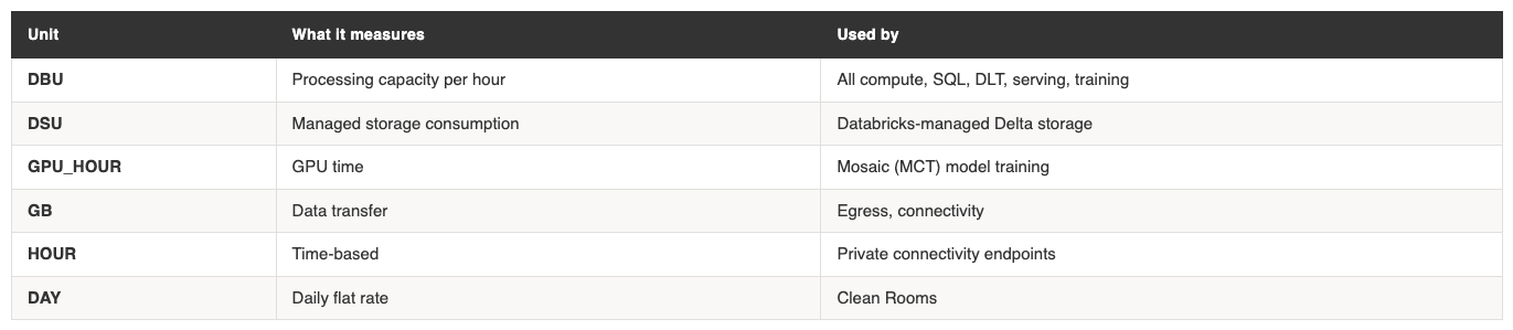
Most Databricks services bill in DBUs, but not all. Databricks uses six distinct billing units across its product surface:
For most organisations, DBUs will dominate the bill. But storage and networking costs are easy to overlook, especially in architectures that use cross-region replication or Delta Sharing. These show up as DSU and GB charges respectively, and they can become meaningful at scale.
List prices and what you actually pay
Every SKU has a list price, visible in system.billing.list_prices. This is the baseline. Your actual price may differ because of negotiated discounts, promotional pricing, or credits. The system table shows both a default price and an effective_list price. The effective list price reflects promotions. Neither reflects your negotiated rate.
This distinction matters for every dashboard and report you build downstream. Be explicit about which price basis you use. Joining usage to list prices without this context will produce numbers that don’t match your invoice.
What generated the cost vs how it’s priced
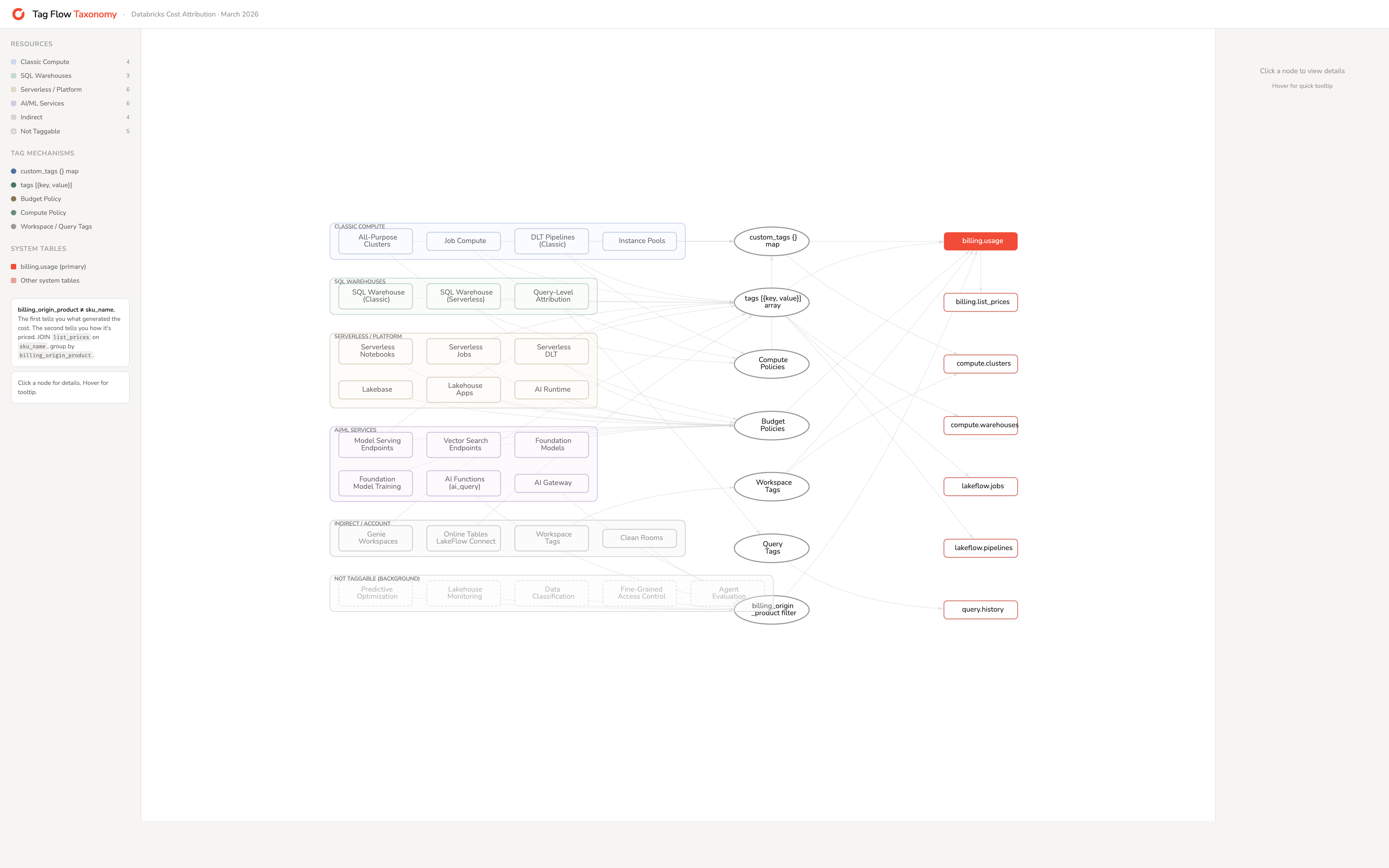
There is a second distinction that is equally important and far less obvious. Every record in system.billing.usage has two fields that look like they should tell you the same thing but don’t: billing_origin_product and sku_name.
billing_origin_product tells you what generated the cost. Vector Search, Predictive Optimization, AI Functions, Lakehouse Apps. It is the service that consumed the resource.
sku_name tells you how that consumption is priced. It maps to a row in system.billing.list_prices. It is the billing meter.
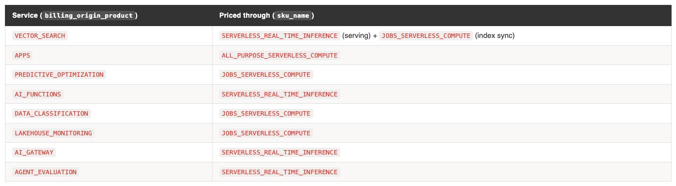
These are different dimensions. Many services do not have their own SKU. They bill through an existing one:
This has three practical consequences:
You will not find these services in list_prices. If you query list_prices for a “Vector Search” SKU, you get nothing. The price is the regional SERVERLESS_REAL_TIME_INFERENCE rate.
Grouping by sku_name alone hides what’s driving cost. Your “serverless jobs” spend might actually be Vector Search index maintenance, Predictive Optimization, or Data Classification running in the background. Always include billing_origin_product in your cost reports.
A single service can bill through multiple SKUs. Vector Search uses SERVERLESS_REAL_TIME_INFERENCE for endpoint serving and JOBS_SERVERLESS_COMPUTE for index sync. Lakebase uses DATABASE_SERVERLESS_COMPUTE for queries, DATABRICKS_STORAGE for persistence, and JOBS_SERVERLESS_COMPUTE for maintenance. One service, three billing lines.
The cost landscape table in the next section is organised by billing_origin_product. The price column shows which sku_name applies.
2. The cost landscape: every service and what it costs
For: Everyone
The table below maps every Databricks service to its SKU, billing unit, and current list price. Prices are from system_union.billing.list_prices as of March 2026, USD. Regional variants are collapsed to ranges.
Compute
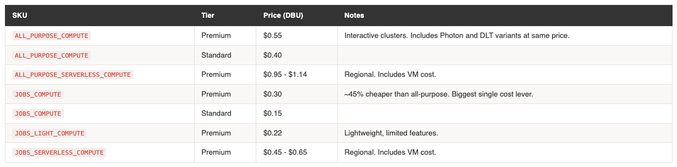
Job compute at $0.30/DBU vs all-purpose at $0.55/DBU is the single largest cost optimisation available to most teams. If a workload can run as a job, it should.
Serverless compute appears more expensive ($0.45-$0.65 vs $0.30 for classic jobs), but the comparison is misleading. Serverless pricing includes the VM cost. Classic compute pricing does not. Your cloud provider bills you separately for the underlying VMs. The true cost comparison depends on your VM sizing and utilisation.
SQL Warehouses
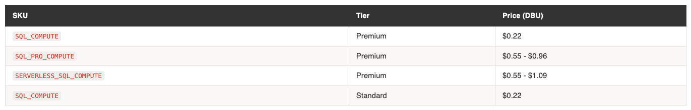
Classic SQL at $0.22 is flat across regions. Pro and serverless are regional. The jump from classic to Pro ($0.22 → $0.55+) is significant. Know which tier your warehouses are running.
DLT / Lakeflow Pipelines
DLT pricing is tier-based, not region-based. Core ($0.30) is the same as job compute. Pro ($0.38) adds CDC and expectations. Advanced ($0.54) adds flow-level lineage. Photon variants exist at the same price points. Standard tier is identical to Premium for DLT.
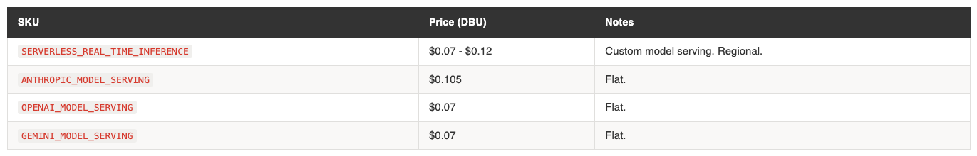
AI/ML Serving
Foundation model APIs bill in DBUs, not per token, in the list prices table. The per-token cost is derived from how many DBUs a given model consumes per request.
Vector Search
Vector Search has three billing components. The endpoint that serves queries bills through the inference SKU. The background process that syncs the index from the source Delta table bills as serverless jobs. And the index itself incurs storage costs as DSU, with a minimum of 4GB per endpoint regardless of actual index size. All three lines carry billing_origin_product = 'VECTOR_SEARCH' but at different prices because the sku_name differs.
The index sync cost deserves particular attention because it depends on the trigger configuration. If Delta Sync is set to continuous, the sync process runs permanently and bills continuously at the serverless jobs rate ($0.45-$0.65/DBU). If set to triggered (on-demand), it runs only when explicitly invoked or on a schedule. For tables with infrequent updates, triggered sync is significantly cheaper. For tables with high write frequency where freshness matters, continuous sync is appropriate but the cost scales with both table size and write volume. This is one of the most common sources of unexpectedly high Vector Search bills.
AI Services
AI Functions deserve specific attention. Every ai_query() call in a SQL query or notebook bills through the inference SKU. On a shared SQL warehouse running dashboards that use ai_query(), this can be a significant and unexpected cost driver because it’s not visible in the warehouse’s DBU consumption — it appears as a separate billing line with billing_origin_product = 'AI_FUNCTIONS'.
Model Training
Lakebase
Lakebase is Databricks’ managed PostgreSQL-compatible database, now GA. The effective list price is roughly 50% of the default price. This is a promotional rate that has carried through from preview into GA, so it is the actual price you should use for cost estimation.
Lakebase billing is purely serverless. There is no provisioned capacity option. Costs scale with query volume and complexity. In addition to the compute DBU charge, Lakebase also incurs DATABRICKS_STORAGE (DSU) for data persistence and JOBS_SERVERLESS_COMPUTE for background maintenance tasks. These show up as separate billing lines with billing_origin_product = 'LAKEBASE', so you can filter and track the full cost of the service.
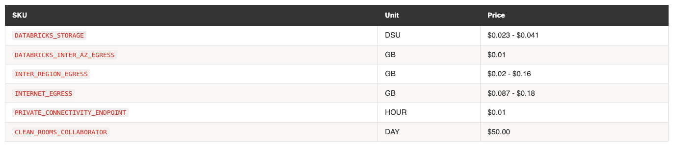
Storage, Networking, Other
Networking costs add up with Delta Sharing and cross-region replication. Inter-region egress at $0.02-$0.16/GB is worth monitoring if your architecture spans regions.
Platform & Background Services
These services run automatically or in the background. They have no dedicated SKU — they bill through existing serverless SKUs. Because they lack dedicated pricing, they are easy to overlook. But collectively, they can account for meaningful spend.Predictive Optimization is the one to watch. It runs continuously in the background once enabled, compacting and optimising tables. In an account with many tables, this becomes a visible line item. You can track it by filtering billing_origin_product = 'PREDICTIVE_OPTIMIZATION' and decide whether the optimisation benefit justifies the cost per catalog.
Data Classification is similar — automatic scanning that bills as serverless jobs. If you’ve enabled it on large catalogs, check the spend.
3. Tagging: what you can tag and how
For: Developers, Platform Engineers
Cost attribution in Databricks comes down to one thing: getting the right tags onto the right resources so they appear in system.billing.usage.custom_tags. This section covers what you can tag, how to tag it, and where tags end up.
An entire overview (to be published soon as interactive HTML) of the various component and how they appear and where:
Classic compute resources
All-purpose clusters are the most straightforward. Set custom_tags as a key-value map when creating or editing the cluster. Available in the UI (Compute → Advanced → Tags), via the Clusters API, Terraform (databricks_cluster.custom_tags), and DABs (clusters[].custom_tags). Tags take effect at cluster start and require a restart to update.
Job clusters accept tags at two levels. The job definition has a tags map (max 25) that propagates to any job clusters created during runs. The new_cluster spec within a job also accepts custom_tags. Both flow into billing records. Databricks auto-applies RunName and JobId as default tags on every job cluster.
DLT pipelines accept tags at the pipeline level (max 25, Public Preview) and at the cluster level within the pipeline spec. Pipeline tags are forwarded to the underlying clusters. DLT has three pricing tiers: Core ($0.30/DBU), Pro ($0.38), and Advanced ($0.54). The SKU in your billing records tells you which tier is running.
Instance pools use the same custom_tags map (max 43 on AWS). This matters more than it might seem. On AWS and Azure, when a cluster launches from a pool, only pool and workspace tags propagate to cloud resources. Cluster tags do not. If your finance team uses AWS Cost Explorer or Azure Cost Analysis, cost attribution tags must be on the pool, not the cluster.
SQL warehouses
SQL warehouses use a different tag structure from clusters. The API expects a tags object containing a custom_tags array of {key, value} objects. In Terraform, this becomes a nested block syntax:
This structural difference from clusters is a common source of configuration errors when teams write Terraform modules that try to handle both.
For query-level attribution on shared warehouses, use query tags: SET QUERY_TAGS['team'] = 'marketing'. These appear in system.query.history.query_tags (Public Preview) and enable proportional cost allocation across teams sharing a warehouse.
Serverless resources
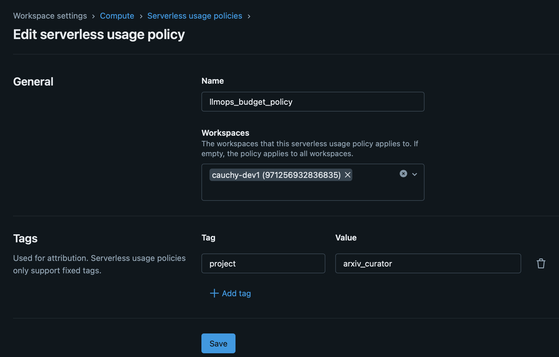
Serverless compute runs on Databricks-managed infrastructure. There are no cloud resources in your account to tag. The tagging mechanism is the serverless budget policy.
A budget policy defines custom tag key-value pairs (max 20). You assign the policy to users, groups, or service principals. When an assigned user runs a serverless workload, the policy’s tags appear in system.billing.usage.custom_tags and the policy ID is stored in usage_metadata.budget_policy_id.
Budget policies apply to: serverless notebooks, serverless jobs, serverless pipelines, model serving endpoints, and Vector Search endpoints.
- If a user has only one policy assigned, it auto-applies to new serverless resources.
- If multiple policies are assigned, the user must choose. Default is alphabetical first.
- If a notebook runs inside a job, the job’s budget policy applies. The notebook’s policy is ignored.
- Pipeline tag updates in Development mode take 24 hours to propagate.
AI/ML services
Model serving endpoints accept both tags (array of {key, value}) and a budget_policy_id. Tags auto-propagate to billing logs. Available in the UI, API, Terraform, and DABs.
Vector Search endpoints support only budget_policy_id. No direct custom tags. Both the serving component (SERVERLESS_REAL_TIME_INFERENCE SKU) and the index sync component (JOBS_SERVERLESS_COMPUTE SKU) carry billing_origin_product = 'VECTOR_SEARCH', so you can filter for all Vector Search costs. The endpoint’s budget_policy_id propagates to the serving lines. The index sync lines also carry the budget_policy_id.
Foundation model APIs (Anthropic, OpenAI, Gemini) bill through the serving endpoint. Tag the endpoint.
AI Functions, AI Gateway, Agent Evaluation — These services bill through SERVERLESS_REAL_TIME_INFERENCE and are not directly taggable. AI Functions (ai_query() calls) inherit context from the SQL warehouse or notebook that invoked them. To attribute these costs, filter by billing_origin_product and correlate with the workspace and time window.
Platform services that are not taggable
Several background services generate cost but have no tagging surface:
Predictive Optimization — bills as JOBS_SERVERLESS_COMPUTE. Not taggable. Attribute by billing_origin_product.
Data Classification — bills as JOBS_SERVERLESS_COMPUTE. Not taggable. Attribute by billing_origin_product.
Lakehouse Monitoring — bills as JOBS_SERVERLESS_COMPUTE. Auto-tagged with LakehouseMonitoringTableId and related keys.
Lakehouse Apps — bills as ALL_PURPOSE_SERVERLESS_COMPUTE. Supports budget_policy_id. Identified via usage_metadata.app_name.
Fine-Grained Access Control — bills as JOBS_SERVERLESS_COMPUTE. Not taggable. Attribute by billing_origin_product.
For these services, billing_origin_product is the only reliable cost attribution mechanism. Include it in every cost report.
Workspace-level tags
Workspace tags propagate to all compute within the workspace. Set via the Account API or Azure ARM resource group tags. Useful for account-wide defaults like org or account_id. Propagation takes up to one hour, and existing resources need a restart.
4. Tag enforcement: from optional to mandatory
For: Platform Engineers
Tags only work for cost attribution if they’re consistently applied. Left to individual developers, tagging is inconsistent. Platform teams need enforcement mechanisms.
Compute policies
Compute policies are the strongest enforcement lever for classic compute. They control what developers can and cannot configure when creating clusters. For tags, three policy types matter:
"type": "fixed" — sets an immutable value. Users cannot change it. Use for tags that should always be the same within a policy (e.g. team name).
"type": "unlimited" — requires the tag but allows any value. Use for tags where users need to provide input (e.g. project name).
"type": "allowlist" — restricts to a predefined set. Use for cost centers or environments where values must match your finance taxonomy.
If a user tries to create a cluster without a required tag, creation fails. This is the enforcement. No tag, no cluster.
One limitation: there is no equivalent enforcement for job-level tags. Compute policies apply to clusters, not jobs. Job tags cannot be made mandatory through policy controls.
Serverless budget policies
For serverless compute, budget policies are the enforcement mechanism. Create policies with the required tags, assign them to users or groups, and serverless usage gets tagged automatically. The platform team’s job is to ensure every user has an appropriate policy assigned.
Enforcement maturity
A practical progression:
Crawl — Recommend tags. Report on untagged percentage. No enforcement.
Walk — Enforce via compute policies. Create budget policies for serverless. Monitor compliance.
Run — Deny untagged compute via IAM-level controls (AWS). Achieve >90% allocation coverage.
Track “allocated %” as a governance KPI. It tells you what fraction of your spend can be attributed to an owner. Start measuring it early.
5. Reading the bill: system tables for cost attribution
For: Developers, Platform Engineers
The core join
Everything starts with system.billing.usage joined to system.billing.list_prices. Get this join wrong and every downstream number is wrong.
SELECT
  u.billing_origin_product,
  u.sku_name,
  u.usage_date,
  u.custom_tags,
  u.usage_quantity AS dbus,
  u.usage_quantity * lp.pricing.effective_list.default AS estimated_cost
FROM system.billing.usage u
JOIN system.billing.list_prices lp
  ON lp.sku_name = u.sku_name
  AND u.usage_end_time >= lp.price_start_time
  AND (lp.price_end_time IS NULL OR u.usage_end_time < lp.price_end_time)
WHERE u.usage_date >= DATE_TRUNC('month', CURRENT_DATE)
Two things to get right here:
The time-window logic (price_start_time / price_end_time) is essential. Without it, you join to multiple price records for the same SKU and inflate your costs. This is the most common cost calculation mistake in Databricks.
Always include billing_origin_product alongside sku_name. As covered in Section 1, these are different dimensions. Joining on sku_name gives you the price, but billing_origin_product tells you what actually consumed it. Without both, your Vector Search costs disappear into your “serverless inference” line and your Predictive Optimization costs hide inside “serverless jobs”.
Tag-based cost aggregation
With tags in place, aggregation is straightforward:
SELECT
  custom_tags['team'] AS team,
  custom_tags['cost_center'] AS cost_center,
  sku_name,
  SUM(usage_quantity) AS total_dbus,
  SUM(usage_quantity * lp.pricing.effective_list.default) AS estimated_cost
FROM system.billing.usage u
JOIN system.billing.list_prices lp
  ON lp.sku_name = u.sku_name
  AND u.usage_end_time >= lp.price_start_time
  AND (lp.price_end_time IS NULL OR u.usage_end_time < lp.price_end_time)
WHERE usage_date >= DATE_TRUNC('month', CURRENT_DATE)
  AND custom_tags['team'] IS NOT NULL
GROUP BY 1, 2, 3
ORDER BY estimated_cost DESC
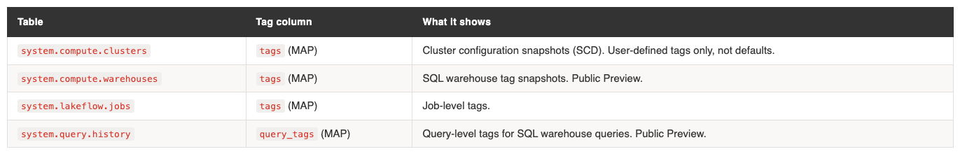
Other tag-bearing system tables
Beyond billing, four system tables carry tag information:
These enable auditing: “what were the tags at the time?” vs “what are the tags now?”
The attribution gap
Jobs running on all-purpose clusters have no job_id in billing records. The cost attributes to the cluster, not the job. There is no way to distinguish which job consumed what on a shared all-purpose cluster. Which you shouldn’t anyway. Even when running the job from Azure Data Factory.
The recommendation: use dedicated job compute or serverless compute for workloads that need per-job cost attribution.
Global vs regional system tables
system.billing.usage is global.Same data regardless of which metastore you query.
system.access.audit is regional for workspace level events, and global for account level events. It’s scoped to the metastore. If you have multiple metastores (one per region), each region’s usage table only shows that region’s data.
This creates a problem for any organisation with multiple regions or cloud providers. Your dashboard in eu-west-1 cannot easily see us-east-1 activity. There is no built-in single pane of glass.
6. Multi-metastore: bridging the visibility gap
For: Platform Engineers
The problem
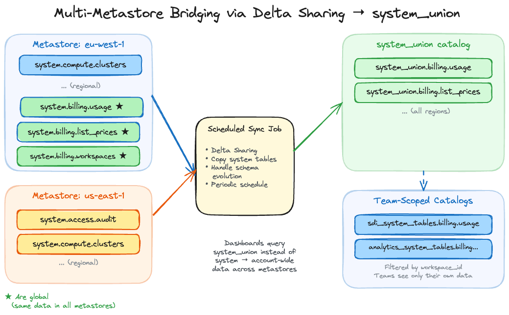
One metastore per region. Some system tables are scoped to the region, and you can only have one metastore per region. A dashboard in one region cannot query another region’s audit table. For organisations operating across multiple regions, or across AWS and Azure, cost visibility is fragmented and it is insightful to combine the system tables for a complete overview.
Why a copy job, not Delta Sharing directly
The natural instinct is to use Delta Sharing to share system tables across metastores. But system tables are managed by Databricks and cannot be shared via Delta Sharing directly. Trying to circumvent it with a VIEW will technically allow you to create the share, only to result in an error when you want to consume it.
The workaround we found is a scheduled job that reads from the system tables in each metastore and writes the data into a regular Delta table in a central catalog, which is than shared. This shared catalog is then combined in a UNION VIEW in acentral catalog, we call system_union, follows the same schema structure as the native system tables (system_union.billing.usage, system_union.billing.list_prices, etc.). The job runs every few hours and does a simple merge based on the changes in the last window. Because the data is now in a regular Delta table that you own, it can be shared via Delta Sharing to other metastores, or queried directly if the central catalog is accessible. Benefit of only changing the catalog name is that the dashboards allow easy parametrisation of the catalog name and as such you have to change little.
The system table schema changes occasionally as Databricks adds columns or modifies types. The sync job needs to handle schema evolution, which is a known maintenance cost. In practice this means catching schema mismatches on the merge and evolving the target table accordingly.
The unified catalog serves a second purpose beyond cross-metastore visibility. By creating filtered views on top of it, you can produce team-specific catalogs that contain only the system table entries relevant to that team’s workspaces. Team “SDI” gets sdi_system_tables.billing.usage showing only their workspaces. They see their costs without access to the full account view.
This serves three purposes: access control (teams see only their own data), simplicity (a developer doesn’t need to understand the full account structure to see their costs), and dashboard personalisation (the same dashboard template, pointed at a team-scoped catalog, becomes a tailored cost view for that team without any modification to the dashboard itself).
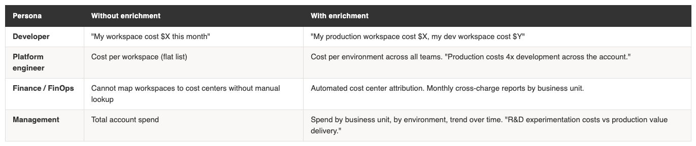
The system.billing.workspaces table contains workspace names and IDs, but no environment label, team, region, or cost center. The workspace is one of the most natural aggregation dimensions for cost reporting, yet the raw table lacks the metadata to make those aggregations useful.
Enrichment adds those missing columns so that every billing record can be joined to structured metadata about which team, environment, and business unit a workspace belongs to. Once enriched, workspaces become a first-class dimension in your cost model.
Parse naming conventions. If your workspaces follow a consistent pattern like team-environment-region (e.g. sdi-production-westeurope), you can split the name into separate columns using string functions. This is the cheapest approach but depends on naming discipline. In practice, most organisations have partial consistency at best, and edge cases (renamed workspaces, legacy naming) require manual overrides.
Pull cloud provider tags. On Azure, workspace-level tags set through ARM resource groups contain metadata that Databricks doesn’t expose in its system tables. You can query the Azure Resource Graph API to retrieve these tags and join them to the workspaces table. This works well if your cloud team already maintains tagging standards on Azure resources. On AWS, similar metadata can be retrieved via the AWS Resource Groups Tagging API.
Maintain a mapping table. A manually curated Delta table that maps workspace IDs to team, environment, cost center, and any other business dimensions. This is the most reliable approach because it doesn’t depend on naming conventions or cloud provider tags being correct, but it requires ongoing maintenance. The mapping table should be treated as a governed asset with clear ownership.
What enrichment unlocks per team:
The enriched workspace table becomes a dimension table that you join to system.billing.usage via workspace_id. Combined with custom tags on resources, it gives you two independent attribution paths: tags for workload-level attribution (which job, which team tagged the cluster) and workspace enrichment for organisational-level attribution (which business unit owns this workspace, what environment is it).
A practical pattern is to create the enriched table as a view in your system_union catalog:
CREATE OR REPLACE VIEW system_union.billing.workspaces_enriched AS
SELECT
  w.*,
  CASE
    WHEN w.workspace_name LIKE '%-production-%' THEN 'production'
    WHEN w.workspace_name LIKE '%-dev-%' THEN 'development'
    WHEN w.workspace_name LIKE '%-staging-%' THEN 'staging'
    ELSE COALESCE(m.environment, 'unknown')
  END AS environment,
  COALESCE(m.team, split(w.workspace_name, '-')[0]) AS team,
  COALESCE(m.cost_center, 'unassigned') AS cost_center
FROM system_union.billing.workspaces w
LEFT JOIN workspace_metadata.default.workspace_mapping m
  ON w.workspace_id = m.workspace_id
This combines naming convention parsing with a manual mapping fallback. The COALESCE pattern ensures you get a value even when the mapping table has gaps, while the mapping table takes precedence where it exists. The enriched view then works as a drop-in replacement in any dashboard or report that currently joins to the raw workspaces table.
This enrichment is highly custom per organisation. The right approach depends on your naming conventions, cloud provider, and how much maintenance effort your team can sustain. But without it, you are limited to aggregating at the workspace level, which is rarely the dimension that finance teams need for cross-charging.
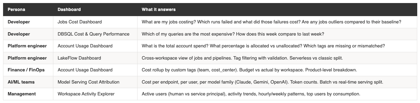
7. Dashboards: from system tables to actionable views
System tables and tags are the foundation. Dashboards are what people actually look at. The goal is a set of views where each persona can answer their questions without needing to write SQL. Below is an aggregation of the most frequently shared dashboards.
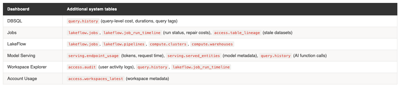
All dashboards share the same billing.usage + list_prices join as their cost calculation core. Each adds domain-specific system tables:
Tag matching analysis
The Account Usage Dashboard v3 includes a dedicated Tag Matching Analysis page. It identifies:
Usage records with no custom tags (completely unattributable)
Records with tags that don’t match expected values (e.g. a cost_center value that doesn’t exist in your taxonomy)
The “allocated %” metric: what fraction of total spend has a valid owner tag
This is the operational view for the “enforcement maturity” discussed in section 4. As you roll out tagging policies, this dashboard shows whether they’re working.
Failed run costs: a hidden cost driver
The Jobs dashboard tracks something most cost reports miss: the cost of failed runs. A job that fails after 45 minutes of compute still incurs the full DBU cost for that time. If it retries automatically, the repair run adds more.
The dashboard surfaces: - Cost per job broken down by result state (succeeded, failed, timed out) - Most-repaired jobs in the last 30 days and their cumulative repair cost - Outlier runs that exceeded the P90 baseline cost for that job
This is operational insight that finance teams rarely see but should. A job with a 15% failure rate and automatic retries can silently inflate costs by 20%+.
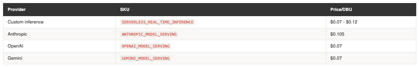
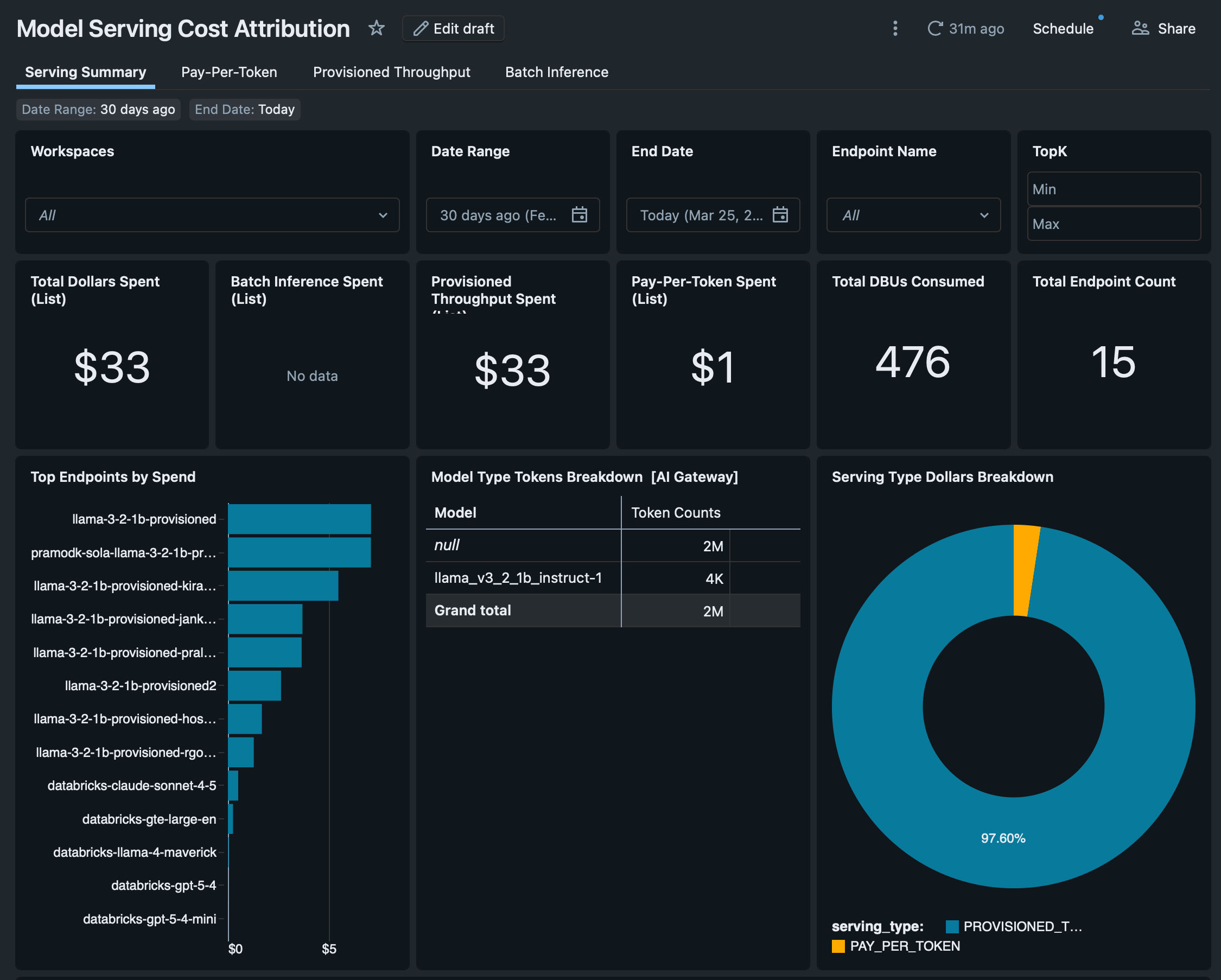
Model serving cost by model family
The Model Serving dashboard breaks down serving costs by provider. Foundation model APIs each have their own SKU:
The dashboard also tracks batch inference costs across executing compute types (DBSQL, DLT, jobs, all-purpose clusters), showing where AI workloads actually run and what they cost. For organisations using AI functions in SQL (ai_query, ai_classify), the dashboard pulls these from query.history to attribute AI costs incurred through SQL warehouses.
Catalog convention
All dashboards are adjusted now to work with a configurable default catalog. If you use the system_union catalog convention from section 6, swap the default catalog name and the dashboards show account-wide data across metastores. If you use team-scoped catalogs, each team gets their own dashboard view automatically.
8. Cost allocation and reporting: the finance perspective
For: Finance / FinOps, Management
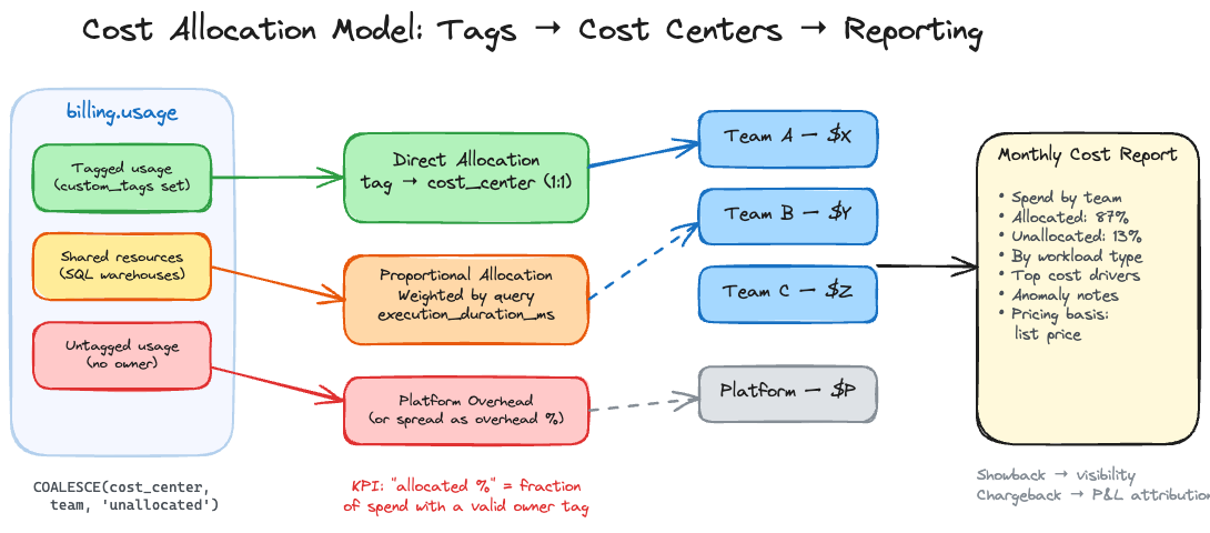
Showback vs chargeback
Two terms finance teams will recognise:
Showback reports costs by team, product, or department for visibility and behavioural change. No general ledger movement. The spend stays in a centralised budget. The goal is accountability through transparency.
Chargeback sends costs to business unit budgets or product P&Ls with formal reconciliation and month-end processes. It requires agreed allocation policy, high tag coverage, and a repeatable close process.
Showback is always required. Chargeback depends on organisational accounting policy. Neither is inherently more mature. Start with showback. Graduate to chargeback when finance and engineering agree on allocation rules.
Allocation models
Direct allocation is the best case. Each billing record maps to one owner via custom tags. Define an allocation key:
COALESCE(
  custom_tags['cost_center'],
  custom_tags['team'],
  'unallocated'
) AS allocation_key
Track “unallocated %” as a governance KPI. It tells you what fraction of spend has no owner. Reduce it over time.
Proportional allocation is necessary for shared resources. A SQL warehouse serving multiple teams can’t be directly allocated. Split the warehouse cost using query execution time from system.query.history:
-- Proportional allocation for shared SQL warehouse
WITH warehouse_cost AS (
  SELECT
    usage_metadata.warehouse_id,
    SUM(usage_quantity * lp.pricing.effective_list.default) AS total_cost
  FROM system.billing.usage u
  JOIN system.billing.list_prices lp
    ON lp.sku_name = u.sku_name
    AND u.usage_end_time >= lp.price_start_time
    AND (lp.price_end_time IS NULL OR u.usage_end_time < lp.price_end_time)
  WHERE sku_name LIKE '%SQL%'
  GROUP BY 1
),
query_weights AS (
  SELECT
    compute.warehouse_id,
    query_tags['team'] AS team,
    SUM(execution_duration_ms) AS team_duration
  FROM system.query.history
  WHERE query_tags['team'] IS NOT NULL
  GROUP BY 1, 2
)
SELECT
  qw.team,
  wc.total_cost * (qw.team_duration / SUM(qw.team_duration) OVER (PARTITION BY qw.warehouse_id)) AS allocated_cost
FROM query_weights qw
JOIN warehouse_cost wc ON qw.warehouse_id = wc.warehouse_id
Hybrid allocation is the most common mature pattern. Direct allocate everything with a valid tag. Proportionally allocate shared resources. Attribute the remainder to a platform cost center and optionally spread it as overhead.
What a monthly cost report should contain
Spend summary by cost center or team, with allocated vs unallocated percentage
Spend by workload type (compute, SQL, DLT, serving) to show where growth is
Top cost drivers: workspaces, clusters, jobs, warehouses ranked by spend
Pricing basis disclosure: explicitly state whether numbers use list prices or negotiated rates
Anomaly notes: spikes with driver explanations and remediation actions
Budget governance
Databricks budgets track spending against a monthly threshold and send email alerts. They do not stop usage or charges. The final bill can exceed the budget amount. Emails can lag up to 24 hours. Budgets use list prices, not negotiated rates.
For faster, more flexible alerting, use SQL alerts on system.billing.usage queries delivered via Slack or webhook notification destinations. A burn-rate alert that fires when daily spend exceeds a threshold is more useful than a monthly budget email that arrives after the fact.
Hard spending limits do not exist natively. The enforcement lever is compute policies: restrict what can be created, by whom, and at what size. Capacity control, not spending caps.
9. Putting it together
For: Everyone
Common mistakes
Treating budgets as hard stops. They are alerts, not controls. If your governance model assumes budgets prevent overspend, it will fail.
Starting tagging late. Tags cannot be applied retroactively to historical billing records. Every day without tags is a day of unattributable spend.
Assuming tags propagate uniformly. Pool-backed clusters on AWS/Azure don’t pass cluster tags to cloud resources. Serverless resources need budget policies, not cluster tags. Different resources have different tag structures.
Incorrect list_prices joins. Without the time-window logic on price_start_time and price_end_time, you join to multiple price records per usage line and inflate your numbers.
Ignoring cloud infrastructure costs. DBU costs are only part of the bill. The VMs, storage, and networking underneath are billed separately by your cloud provider. Serverless pricing includes the VM cost. Classic compute pricing does not.
Do this first
Define a tag taxonomy. Four tags cover most needs: cost_center, team, environment, product. Standardise the allowed values.
Enforce tags. Compute policies for classic compute. Budget policies for serverless. No tag, no cluster.
Build the allocation dataset.system.billing.usage joined to system.billing.list_prices with correct time-window logic. State the pricing basis.
Set up alerting. SQL alerts on daily spend anomalies, delivered to Slack. Don’t rely on budget emails.
Report monthly. Spend by owner, by workload type, with allocated percentage and anomaly explanations.
Iterate. Graduate from showback to chargeback when allocation coverage is high enough and finance agrees on the rules.
Companion notebook
This guide is accompanied by a Databricks notebook that demonstrates how to tag every resource type programmatically. It uses the Databricks SDK for compute-layer tagging (clusters, jobs, warehouses, pipelines, budget policies, compute policies) and Brickkit for Unity Catalog and AI/ML asset tagging (catalogs, schemas, tables, Vector Search, Genie spaces, model serving). The notebook is structured to be run cell-by-cell as a tagging workshop.
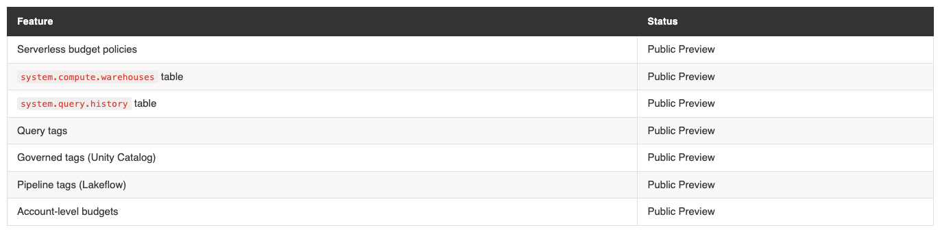
Features in Public Preview (March 2026)
Several capabilities referenced in this guide are in Public Preview and may change:
Thanks for reading Cauchy's stories! Subscribe for free to receive new posts and support my work.